Coronavirus Data, Analysis

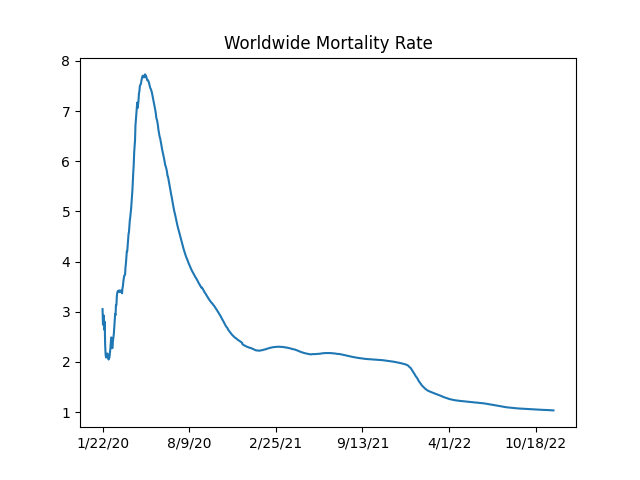
Mortality Rate

Fatality / Cases ratio is around 2.2%, the cases is for people with symptoms. What would be the fatality rate for the broader population? On one of those cruise ships which experienced the epidemic in an isolated environment, they found about 1/3 rd of the people were infected. We can assume the virus reached everyone possible on that ship. 1/3 of mortality rate is nearly 1%. So if given the chance, covid can kill 1% of an entire population. As a reference point, annual growth of world population hovers around the same ratio

Code is from [2]

import util
world_rate_df = util.mortality_rate()
world_rate_df['deaths / 100 confirmed'].plot(title='Worldwide Mortality Rate')
plt.savefig('mort.png')

11/25/22    1.034779
11/26/22    1.034415
11/27/22    1.034074
11/28/22    1.033569
Name: deaths / 100 confirmed, dtype: float64

The SIR Model

$$ \frac{ds}{dt} = -\beta s i $$

$$ \frac{di}{dt} = \beta s i - \gamma i $$

$$ \frac{dr}{dt} = \gamma i $$

Where does $R_0$ come from? Epidemic occurs if # of infected ppl increase, meaning $di / dt > 0$. That means (from second eq above)

$$ \beta si - \gamma i > 0 \implies \frac{\beta s i }{\gamma} > i $$

Then,

$$ \frac{\beta s }{\gamma} > 1 $$

At the beginning of the epidemic everyone is susceptible, so $s \approx 1$. Substitute $s=1$

$$ \frac{\beta}{\gamma} = R_0 > 1 $$

To find $R_0$ from data, we fit the differential equation system above to data, and using the found $\beta$ and $\gamma$ we calculate $R_0$.

Graphs

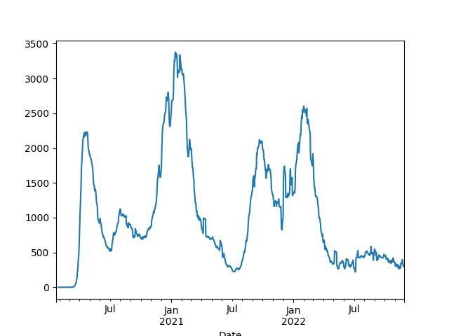
US Daily Deaths, 7-Day Moving Average

import util, pandas as pd
df = util.get_data_combined()
df1 = df[(df['Country/Region']=='US')&(df.index > '2020-01-01')]
df1['New deaths'] = df1['New deaths'].rolling(7).mean()
print (df1['New deaths'].tail(5))
df1['New deaths'].plot()
plt.savefig('US-deaths.png')

Date
2022-11-24    357.571429
2022-11-25    302.428571
2022-11-26    301.000000
2022-11-27    301.000000
2022-11-28    313.285714
Name: New deaths, dtype: float64

FR Daily Deaths, 7-Day Moving Average

import util, pandas as pd
df = util.get_data_combined()
df1 = df[(df['Country/Region']=='France')&(df.index > '2020-01-01')]
df1['New deaths'] = df1['New deaths'].rolling(7).mean()
print (df1['New deaths'].tail(5))
df1['New deaths'].plot()

Date
2022-11-24    68.857143
2022-11-25    68.000000
2022-11-26    68.000000
2022-11-27    68.000000
2022-11-28    61.857143
Name: New deaths, dtype: float64
Out[1]: <AxesSubplot:xlabel='Date'>

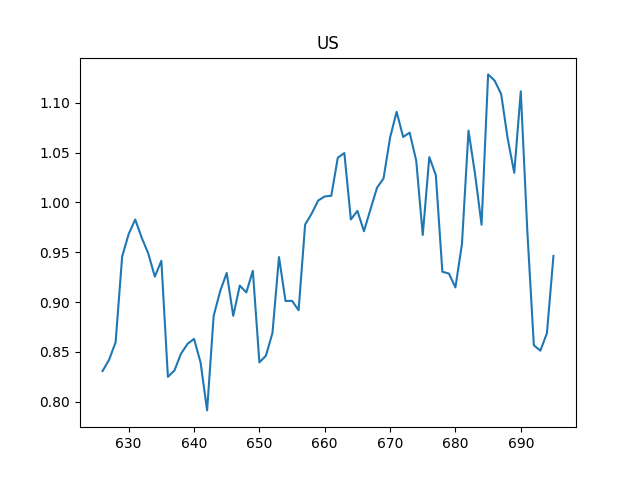
Reproduction Rate $R_t$

This calculation is based on [1]

import util, pandas as pd

df1 = df[(df['Country/Region']=='US')&(df.index > '2021-01-01')]
tau = 7 # length of time window
si_mean = 6.3 # mean of serial interval
si_std = 4.2 # standard deviation of serial interval
conf = 0.95 # confidence level of estimated Reff
c = df1['New cases']
R = util.Reff(c, si_mean, si_std, tau, conf)
df2 = pd.DataFrame(R.T)
print (df2[1].tail(5))
# 0,2 indices 95% conf
df2[1].tail(70).plot()
plt.title('US')
plt.savefig('Rt-US.png')

691    0.971349
692    0.856543
693    0.851197
694    0.868735
695    0.946327
Name: 1, dtype: float64

References

[1] https://github.com/tt-nakamura/Reff.git

[2] https://notebooks.ai/rmotr-curriculum/analyzing-covid19-outbreak-40c03c06

[4] https://web.stanford.edu/~jhj1/teachingdocs/Jones-on-R0.pdf